Transcript
0:00From one to two compartments
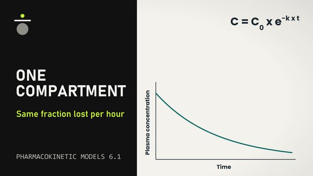
Lesson 6.2 of our pharmacokinetic models module: two compartments. A one-compartment model treats the body as one well-mixed space. Plasma is the liquid part of the blood. In this model, the logarithm of the plasma concentration falls along a straight line after an intravenous dose, an injection into a vein. Half-life is the time for the plasma concentration to fall by half. Elimination is the irreversible loss of drug from the body by metabolism and excretion. For many drugs, the plasma concentration first falls fast and then more slowly.
0:47The two-compartment model
A two-compartment model describes the body as two spaces, and drug moves between them in both directions. The central compartment is the plasma and the organs that the drug reaches fast, such as the liver. The dose enters it, blood samples come from it, and drug leaves the body from it. The peripheral compartment is the tissues that the drug reaches more slowly. Which compartment a tissue belongs to depends on its blood flow and on how easily the drug crosses its cell membranes.
1:25Distribution and elimination phases
The distribution phase is the early, fast fall of the plasma concentration, while drug moves into the peripheral compartment. The elimination phase is the later, slow fall, in which the plasma and tissue concentrations fall in parallel.
1:46The two-exponential equation
The plasma concentration, C, at time t after the dose is the sum of two exponential terms. C equals A times e to the minus alpha t, plus B times e to the minus beta t. Here, e is the number 2.718, the base of the natural logarithm. Alpha and beta are rate constants: the larger the constant, the faster its term falls. Alpha is the larger. A and B are the values of the two terms at time zero. Three points explain this curve: the two slopes, what each phase means in the body, and the half-life of the slow phase.
2:32The two slopes
The first is the two slopes. On a logarithmic scale, each exponential term is a straight line, steep for alpha and shallow for beta. The alpha term soon becomes small, and the curve then lies on the beta line, whose slope gives minus beta. When alpha is much larger than beta, the curve shows two nearly straight phases. Each straight phase usually needs its own compartment in the model.
3:04What each phase means in the body
The second is what each phase means in the body. In the distribution phase, the plasma concentration falls for two reasons: drug moves into the tissues, and the body also eliminates drug. At the same time, the concentration in the tissues rises. In the elimination phase, the ratio of the tissue to the plasma concentration stays constant. As the plasma concentration falls, drug moves back from the tissues into the blood, and the two concentrations fall in parallel.
3:43The terminal half-life
The third is the terminal half-life. It is the half-life of the elimination phase, and it equals 0.693, the natural logarithm of 2, divided by beta. Clearance is the rate of elimination divided by the plasma concentration. The terminal half-life is longer when a larger share of the drug is in the tissues, and shorter when clearance is higher. It is the half-life usually reported for a drug. The distribution half-life is 0.693 divided by alpha.
4:22Digoxin
Digoxin shows the two phases, and why the time of a blood sample matters. Digoxin is a drug for heart failure and for atrial fibrillation, a fast and irregular heart rhythm. Nine healthy men each received single intravenous doses of 0.5, 1 and 1.5 milligrams, with blood samples for 35 hours after each dose. The mean distribution half-life was 0.35 hours, about 21 minutes. The mean terminal half-life was 27.9 hours, about 80 times longer. Digoxin distributes widely into the tissues, and skeletal muscle holds the largest store.
5:13Time of the blood sample
In a second study of 12 healthy men, the effect on the heart followed the calculated concentration in a third, slowly filled compartment. The two-compartment fit of the first study does not show this slower uptake. Distribution of digoxin into the tissues takes 6 to 8 hours. A sample before then gives an unreliable measure of the effect and of toxicity. Blood samples for digoxin are therefore taken at least 6 hours after a dose, or just before the next dose.
5:51Summary
In summary, a two-compartment model joins a central compartment, where the dose enters and blood is sampled, to a slowly reached peripheral compartment. When alpha is much larger than beta, the two exponential terms give two nearly straight phases on a logarithmic scale. Drug moves into the tissues in the distribution phase while elimination continues, and in the elimination phase both concentrations fall in parallel. The terminal half-life, 0.693 divided by beta, comes from the elimination phase. In nine healthy men, digoxin had mean half-lives of about 21 minutes and 27.9 hours. Digoxin distributes into the tissues over 6 to 8 hours, and blood samples are therefore taken at least 6 hours after a dose. This concludes lesson 6.2 on two compartments.
Sources
- Jelliffe RW. Some comments and suggestions concerning population pharmacokinetic modeling, especially of digoxin, and its relation to clinical therapy. Ther Drug Monit. 2012. PMID 22735674
- Yim DS, Choi S. Predicting human pharmacokinetics from preclinical data: volume of distribution. Transl Clin Pharmacol. 2020. PMID 33425799
- Toutain PL, Bousquet-Mélou A. Plasma terminal half-life. J Vet Pharmacol Ther. 2004. PMID 15601438
- Benowitz NL, Meister W. Clinical pharmacokinetics of lignocaine. Clin Pharmacokinet. 1978. PMID 350470
- Cheng JW, Charland SL, Shaw LM, et al. Is the volume of distribution of digoxin reduced in patients with renal dysfunction? Determining digoxin pharmacokinetics by fluorescence polarization immunoassay. Pharmacotherapy. 1997. PMID 9165563
- Mould DR, Upton RN. Basic concepts in population modeling, simulation, and model-based drug development-part 2: introduction to pharmacokinetic modeling methods. CPT Pharmacometrics Syst Pharmacol. 2013. PMID 23887688
- Sahin S, Benet LZ. The operational multiple dosing half-life: a key to defining drug accumulation in patients and to designing extended release dosage forms. Pharm Res. 2008. PMID 19015955
- Ochs HR, Greenblatt DJ, Bodem G, et al. Dose-independent pharmacokinetics of digoxin in humans. Am Heart J. 1978. PMID 358815
- US Food and Drug Administration. LANOXIN (digoxin) injection, prescribing information. 2025. https://dailymed.nlm.nih.gov/dailymed/lookup.cfm?setid=9ec84cac-6ecc-43dc-8006-6ccc029e2707
- Iisalo E. Clinical pharmacokinetics of digoxin. Clin Pharmacokinet. 1977. PMID 322907
- Kramer WG, Kolibash AJ, Lewis RP, et al. Pharmacokinetics of digoxin: relationship between response intensity and predicted compartmental drug levels in man. J Pharmacokinet Biopharm. 1979. PMID 458556
- Mooradian AD. Digitalis. An update of clinical pharmacokinetics, therapeutic monitoring techniques and treatment recommendations. Clin Pharmacokinet. 1988. PMID 3052985
- Kelly RA, Smith TW. Recognition and management of digitalis toxicity. Am J Cardiol. 1992. PMID 1626485
Illustrations adapted from Servier Medical Art (smart.servier.com), CC BY 4.0. Structures drawn with RDKit.