Noncompartmental analysis and population PK
This lesson compares noncompartmental analysis, which needs rich sampling, with population pharmacokinetics, which works with sparse samples. A population analysis of dabigatran in the RE-LY trial shows which tested covariate warrants a change of dose.
Key points
- NCA needs rich sampling, and it calculates the AUC by the trapezoidal rule and the terminal half-life from the log-linear slope.
- Population PK fits one nonlinear mixed-effects model to sparse samples from many patients, and it estimates typical values, between-subject variability and covariate effects.
- For dabigatran, with about three samples per patient, the authors concluded that kidney function is the only tested covariate that warrants a change of dose.
Worked example
Dabigatran
Dabigatran shows how a population PK analysis finds the covariate that needs a change of dose. Dabigatran is an anticoagulant, a drug that reduces the formation of blood clots. Patients take it by mouth as dabigatran etexilate, a prodrug that the body converts to dabigatran. The kidneys excrete most of the dabigatran in the blood unchanged. In the RE-LY trial, patients with atrial fibrillation, a disturbance of the heart rhythm, took 110 or 150 milligrams twice daily. The analysis used 27,706 plasma concentrations from 9,522 patients, about three per patient. A model with two compartments described the data. Age, sex, heart failure, South Asian origin and creatinine clearance, a measure of kidney function, changed the apparent clearance. Body weight and hemoglobin changed the apparent volume of the central compartment, which includes the plasma. At steady state, after repeated twice-daily doses, each covariate other than kidney function changed the exposure by less than 26 percent. A simulation with the model gave the exposure of 75 milligrams twice daily at a creatinine clearance of 15 to 30 milliliters per minute. RE-LY excluded patients with a creatinine clearance this low. The simulated exposure was similar to that of 150 milligrams twice daily at normal kidney function. The authors concluded that, of the covariates tested, only kidney function warrants a change of dose.Equations
- C1, C2
- the two concentrations of a pair of consecutive points
- t2 - t1
- the time between them
- AUC
- the area under the concentration-time curve
- t1/2
- the terminal half-life, the time for the concentration to fall by half in the last phase
- 0.693
- the natural logarithm of 2
- lambda z
- the terminal rate constant, minus the slope of the regression line of the natural logarithm of the concentration against time
- Clast
- the last concentration
- lambda z
- the terminal rate constant
- CL/F
- the apparent clearance, the clearance divided by the bioavailability
- dose
- the oral dose
0:00Concentration-time curves and two methods
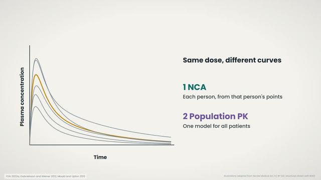
Lesson 6.6 of our pharmacokinetic models module: noncompartmental analysis and population pharmacokinetics. Pharmacokinetics describes what the body does to a drug. In a clinical study, the staff take blood samples at set times after a dose. The drug concentrations in the plasma, the liquid part of the blood, form a concentration-time curve. The area under this curve, AUC, measures the total exposure to the drug. Clearance is the volume of plasma from which the body removes all of the drug per unit of time. Bioavailability is the fraction of the dose that reaches the systemic circulation unchanged. The same dose gives different curves in different patients. Noncompartmental analysis, or NCA, calculates each person's parameters, such as the AUC and the clearance, from that person's points. Population pharmacokinetics, or population PK, fits one model to the data of all patients and explains part of the differences between them.
1:23Noncompartmental analysis
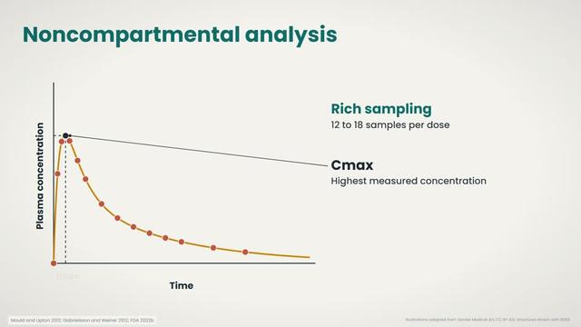
The first method is noncompartmental analysis. It uses no compartments, the spaces of uniform drug concentration in a model, and it makes few assumptions. It needs rich sampling, many samples per person: for most drugs in bioavailability studies, the FDA recommends 12 to 18 for each dose. The highest measured concentration is Cmax, and its time is tmax.
1:57The trapezoidal rule
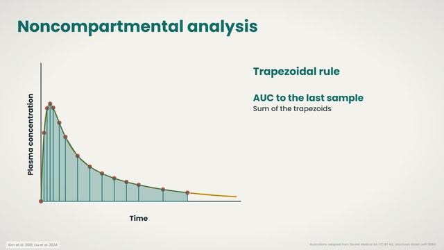
NCA calculates the AUC by the trapezoidal rule. A straight line joins each pair of consecutive points, and the shape under it is a trapezoid. The area of each trapezoid is the mean of its two concentrations times the time between them. The sum of these areas is the AUC to the last sample.
2:24Terminal half-life and AUC to infinity
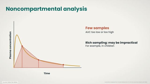
The terminal half-life is the time for the concentration to fall by half in the last phase. On a plot of the natural logarithm of the concentration against time, the points of this phase fall on a straight line. A linear regression line through at least three of these points has a slope of minus lambda z, the terminal rate constant. The terminal half-life is 0.693, the natural logarithm of 2, divided by lambda z. The last concentration divided by lambda z is the area after the last sample, and the two areas together give the AUC to infinity. For an oral dose, the dose divided by this AUC is the apparent clearance, the clearance divided by the bioavailability. With few samples per person, the trapezoidal rule can give an AUC that is too low or too high. Rich sampling may be impractical in some patients, for example in children.
3:39Population pharmacokinetics
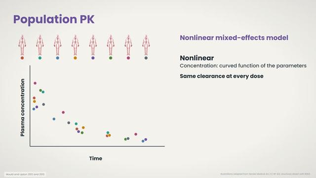
The second method is population pharmacokinetics. It fits a nonlinear mixed-effects model. Nonlinear means that the concentration is a curved function of the parameters, such as an exponential, even when clearance stays the same at every dose.
3:59Fixed and random effects
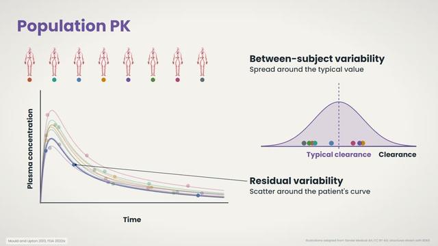
The model mixes two kinds of parameters. Fixed effects have one value for all patients, such as the typical clearance. Random effects describe how far each patient differs from the typical value. Between-subject variability is the spread of the individual values around the typical value. Residual variability is the scatter of the measured points around the model curve of each patient.
4:32Covariates and sparse sampling
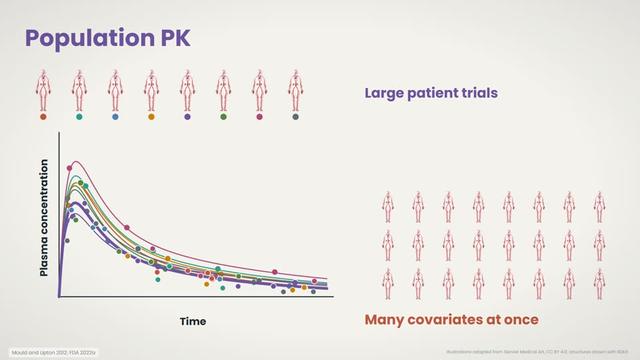
Covariates are measured patient factors, such as body weight or kidney function, that explain part of the between-subject variability. Population PK works with sparse sampling, a few samples from each patient at different times, because it estimates the curve from all patients together. It can therefore use large patient trials and test many covariates at once.
5:02Dabigatran in the RE-LY trial
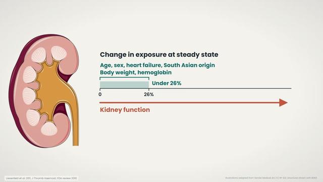
Dabigatran shows how a population PK analysis finds the covariate that needs a change of dose. Dabigatran is an anticoagulant, a drug that reduces the formation of blood clots. Patients take it by mouth as dabigatran etexilate, a prodrug that the body converts to dabigatran. The kidneys excrete most of the dabigatran in the blood unchanged. In the RE-LY trial, patients with atrial fibrillation, a disturbance of the heart rhythm, took 110 or 150 milligrams twice daily. The analysis used 27,706 plasma concentrations from 9,522 patients, about three per patient. A model with two compartments described the data. Age, sex, heart failure, South Asian origin and creatinine clearance, a measure of kidney function, changed the apparent clearance. Body weight and hemoglobin changed the apparent volume of the central compartment, which includes the plasma. At steady state, after repeated twice-daily doses, each covariate other than kidney function changed the exposure by less than 26 percent.
6:34Simulation for kidney function
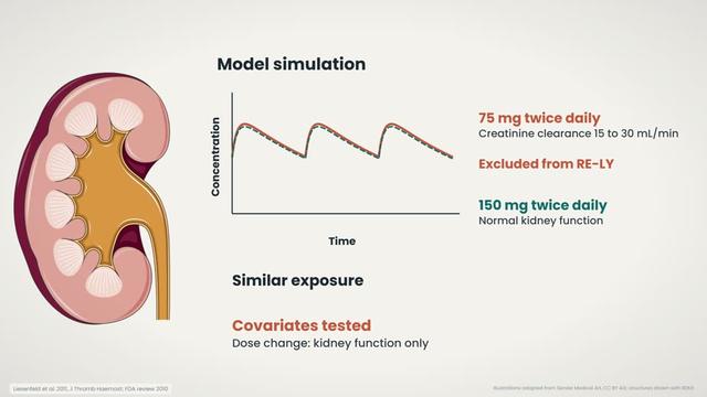
A simulation with the model gave the exposure of 75 milligrams twice daily at a creatinine clearance of 15 to 30 milliliters per minute. RE-LY excluded patients with a creatinine clearance this low. The simulated exposure was similar to that of 150 milligrams twice daily at normal kidney function. The authors concluded that, of the covariates tested, only kidney function warrants a change of dose.
7:09Summary
In summary, NCA needs rich sampling, and it calculates the AUC by the trapezoidal rule and the terminal half-life from the log-linear slope. Population PK fits one nonlinear mixed-effects model to sparse samples from many patients, and it estimates typical values, between-subject variability and covariate effects. For dabigatran, with about three samples per patient, the authors concluded that kidney function is the only tested covariate that warrants a change of dose. This concludes lesson 6.6 on noncompartmental analysis and population pharmacokinetics.
What is noncompartmental analysis?
What is population pharmacokinetics?
How many blood samples does noncompartmental analysis need?
How does noncompartmental analysis calculate the AUC?
How is the terminal half-life calculated from the log-linear slope?
What are fixed effects and random effects?
What is a covariate?
Why can population pharmacokinetics use sparse sampling?
Which covariate of dabigatran warrants a change of dose?
- US Food and Drug Administration. Population pharmacokinetics. Guidance for industry. 2022. https://www.fda.gov/media/128793/download
- US Food and Drug Administration. Bioavailability studies submitted in NDAs or INDs: general considerations. Guidance for industry. 2022. https://www.fda.gov/media/121311/download
- Yim DS. Tutorial for beginners: the concept of clearance explained using the example of a vacuum cleaner. Transl Clin Pharmacol. 2017. PMID 32095451
- Benet LZ, Sodhi JK. Simplifying pharmacokinetics, applying it to drug and dosage form development, and making drug dosage decisions in clinical medicine: the adaptation of Kirchhoff's laws from physics. AAPS J. 2025. PMID 40603610
- Gabrielsson J, Weiner D. Non-compartmental analysis. Methods Mol Biol. 2012. PMID 23007438
- Kim H, Han S, Cho YS, et al. Development of R packages: 'NonCompart' and 'ncar' for noncompartmental analysis (NCA). Transl Clin Pharmacol. 2018. PMID 32055542
- Liu G, Brooks L, Canty J, et al. Deep-NCA: a deep learning methodology for performing noncompartmental analysis of pharmacokinetic data. CPT Pharmacometrics Syst Pharmacol. 2024. PMID 38465417
- Mould DR, Upton RN. Basic concepts in population modeling, simulation, and model-based drug development. CPT Pharmacometrics Syst Pharmacol. 2012. PMID 23835886
- Mould DR, Upton RN. Basic concepts in population modeling, simulation, and model-based drug development-part 2: introduction to pharmacokinetic modeling methods. CPT Pharmacometrics Syst Pharmacol. 2013. PMID 23887688
- Stangier J. Clinical pharmacokinetics and pharmacodynamics of the oral direct thrombin inhibitor dabigatran etexilate. Clin Pharmacokinet. 2008. PMID 18399711
- Escobar C, Barrios V, Jimenez D. Atrial fibrillation and dabigatran: has the time come to use new anticoagulants? Cardiovasc Ther. 2010. PMID 20718760
- Liesenfeld KH, Lehr T, Dansirikul C, et al. Population pharmacokinetic analysis of the oral thrombin inhibitor dabigatran etexilate in patients with non-valvular atrial fibrillation from the RE-LY trial. J Thromb Haemost. 2011. PMID 21972820
- US Food and Drug Administration. Clinical pharmacology and biopharmaceutics review, NDA 22-512 (dabigatran). 2010. https://www.accessdata.fda.gov/drugsatfda_docs/nda/2010/022512Orig1s000ClinPharmR.pdf
Illustrations adapted from Servier Medical Art (smart.servier.com), CC BY 4.0. Structures drawn with RDKit.